Triangulation Analysis

The overall approach in HxMap Triangulation is to perform sequential bundle block adjustments. During each adjustment, a statistical blunder detection is performed, and detected blunders are deactivated in the system. In any case it is recommended to review the triangulation results carefully and - if required - adapt parameterization, change blunder status or re-measure points before repeating the adjustment.

Final results are reached when

• no additional blunders are detected during adjustment compared to previous run

• the RMS values and residuals of ground control points are within expectation

• the estimated Sigma-0 value resulting from the adjustment agrees with the initial sigma-0 a priori.

• the standard deviations of the adjusted terrain points fulfill the requirements of the project

• the RMS values and residuals of GPS and IMU observations are within expectation

To ensure the results produced by the adjustment run present the best possible results, the following criteria should be checked:

• Blunders

• Sigma-0 a-posteriori vs. sigma-0 a priori

• systematic effects at residuals of image points

• quality of adjusted terrain points

• RMS and residuals of ground control points

• RMS and residuals of GPS and IMU observations

HxMap offers a range of tools to support the analysis.

Analyzing the Statistics

Overview section

The Overview section gives a summary of the triangulation block setup and the used image measurements classified into by different kind of point use. The lower section summarizes the expected and estimated Sigma-0 and lists the number of blunders detected during the adjustment run.

Review the resulting Sigma-0 a posteriori. It mainly reflects the remaining errors in the image coordinates, as image measurements usually make up the majority of all observations. Sigma-0 a posteriori needs to be judged in comparison to its initial value. For a well-parameterized triangulation with properly balanced weighting (see variance component scales), the expected and estimated Sigma-0 values should be in the same order.

Decreasing the initial sigma value will generally decrease the final value too. This does not mean the triangulation result becomes 'better'. In other words: Sigma-0 a posteriori is not meaningful by itself but a very useful, overall indicator of the triangulation results quality when compared to sigma-0 a priori!

Variance components

The variance components reflect, if  the GNSS and IMU observations are weighted correctly in respect to other types of observations. A correct weight relation is given, when the variance component for a particular observation type is close to 1.0. The variance component will be less than 1, if the standard deviation a priori is set too large. The variance component will be greater than 1, if the standard deviation a priori is set too small.

The triangulation adjustment report gives an indication on how to properly weight the GNSS/ IMU observations in order to achieve a well parameterized adjustment.

However, a user needs to be aware that a reliable estimation of variance components requires a minimum level of redundancy within the respective group of observations. This redundancy decreases with increased weights, which are influenced by the scale factors provided in the Settings tab, section Variance Components. Increasing the scale factor decreases the weight of an observation and vice versa. If the minimum redundancy isn't achieved, the variance components cannot be reliably estimated. In that case HxMap will display a value of 9.99 for the respective group of observation. In that case it is recommended to decrease the weight of the affected observation group, as the goal is to provide a balanced weighting for all groups of observation in order to get best possible adjustment results. This can be achieved by a slow increase of the corresponding scale factor mentioned above. As soon as the minimum redundancy level is met, the resulting variance components should no longer report a value of 9.99, but a true estimation. Although these resulting variance components may not be in the ideal range, this result would be the best possible for the given block and it's settings.

Ground Points

Review the resulting RMS values for Ground Control and Check Points if they meet your expectations. The Tie Point section allows to analyze the overall achieved accuracy of adjusted Terrain points.

Exterior Orientation

Review the resulting RMS values for photo center coordinates as well as for the orientation angles.

Additional Parameter

This section summarizes the resulting datum and misalignment parameters (RMS values in case of parameterization per sensor or session), if they were enabled for the triangulation run.

Analyzing points

The point tab can also assist for analysis purpose. Get an overview by listing

• Ground Control points with their object residuals

• any tie point by it's number of rays

• tie points by their active/ non-active status

• tie points by their resulting standard deviation

Each of the individual columns in the Points tab is sortable to assist in analysis.

Review Blunders

If the adjustment has classified an image measurement as outlier, the measurement gets marked as a blunder. That means, it was eliminated during the iterative triangulation and has no impact on the results. If the number of remaining measurements (rays) per tie point is below 2, the corresponding tie point gets marked as inactive. The point will no longer be considered in upcoming adjustments, unless the user activates the point measurements again.

If the adjustment has classified a ground control point as an outlier, it is recommended to perform an additional adjustment, which considers only the remaining active ground control points.

Manipulate Tie and Image Points

If desired, a user has the ability to physically delete inactive points or blundered measurements rather than just flag them.

To do so, select the desired points in the Point Tab based on sorting, individual selection or based on a filter and check them. Once points are checked, use the delete option in the toolbar of the Points tab.

In the same way there exists the option to activate or de-activate checked points in order to include or exclude them from a bundle block adjustment run.

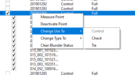
If the intention is to reset the blunder status of image points derived from previous adjustment runs, use "Clear Blunder status..." button. 

It requires a point (measurement) to be checked before use.

A user can also use Context menu on the Points Editor to fastly interact with points:

If you change the point status and do not run immediately some bundle block adjustment, it is important to save these changes so that they will be considered once you come back to the project. Saving the actual settings of a project is done via the "Save Scenario" button:

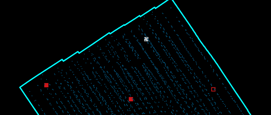
Visualize Points

The map view gives a good overview of all points listed in the points panel. Distinctive styles will indicate the type of point and if the point has been measured or not:

• Check points: triangular shape

• Control points: square shape

• Tie points: round shape

Icons are either filled if they have been measured or empty if they are without measurement.

Colors and sizes for each icon type can be changed either in the HxMap settings or then directly on an individual layer. Points that have been deactivated are shown in a gray color.

Analyze the report

The main toolbar allows the user to review and save the triangulation report. The report includes a protocol of the input parameter, detailed information per processed iteration as well as the results and key statistics collected after adjustment. In case of a hierarchical adjustment run, tabs provide access to the report per subsequent adjustment run based on cardinal view. Go To buttons allow to jump directly to sections of interest, such as Datum shift results or RMS results per Observation group.

Ground Point Statistics

Especially for oblique imagery it is of interest to see the connections of the points (tie points and ground control points) regarding the different cardinal views (Down, North, East, South, West).

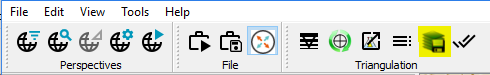
In the Tools menu find the function "Ground Point Statistics". It will open a statistics window as shown below:

Ground Point Statistic - amount of points	Ground Point Statistic - percentages of points

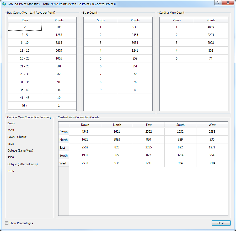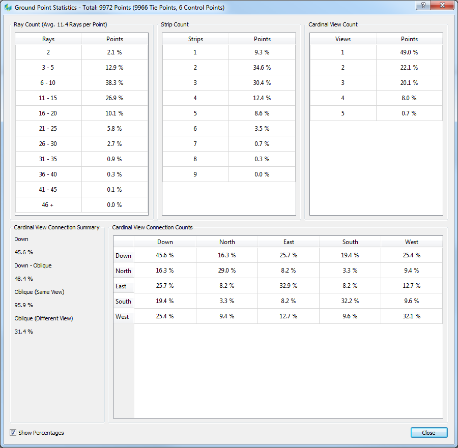Ray Count: lists the number of points measured in a certain number of images (as specified in the Rays column)
Strip Count: lists the number of points measured in 1 to n strips
Cardinal View Count: lists the number of points measured in 1 to 5 cardinal views
Cardinal View Connection Counts: lists the number of points connecting images of different cardinal views

Parallax Analysis

An easy, quick check to verify the quality of the resulting exterior orientation parameter, is to check the quality of the pre-positioning of ground points. To do so, select a ground control point from the Point list, where the location is known and which is preferably not yet measured. Select via a right mouseclick "Measure point". Ideally the ground control location should be displayed in the very center of each image opened within the Measurement window indicating that the determined exterior orientation parameter have a good quality and therefore no obvious parallax is visible.

Graphical Analysis

The results from the last adjustment run are also presented as additional layers in the map view. On the Layers Tab you find the Analysis section, which allows the turn on/off the display of additional analysis layers.

Cell Based Analysis (CBA)

HxMap provides a cell-based analysis which is intended to provide a quick overview on the triangulation quality on the ground. Generally, errors in observables-ground control points, tie points, GNSS/IMU trajectory-will affect the unknown parameters: ground coordinates of tie points and the corrected trajectory.

While the trajectory is important (e.g., to reveal systematic effects) after all a user is interested in ground-based quality measures, since those determine the product accuracy (orthoimage, DTM). Consequently, ground coordinates of tie points should be evaluated, particularly ground space standard deviations and, more meaningful, reliability measures.

Cell based analysis is based on the most reliable point in a cell. For this purpose a reliability indicator is used, which is based on the point with the highest number of rays per cell. The calculated a-posteriori standard deviation for that point is used to determine the quality for the cell. The quality is represented by a color scale ranging from green (good) to red (bad quality). In case the complete project is represented in red, review all your input data and parameterization. In case single cells are represented in red, it most likely indicates a non-sufficient tie point distribution or connectivity, e.g. for images at the very edge of the project. Check, if there's an obvious reason such as water coverage. If that is not the case, you may want to add additional tie points.

Sample for Cell based Analysis illustrating the effects described in the sequence above:

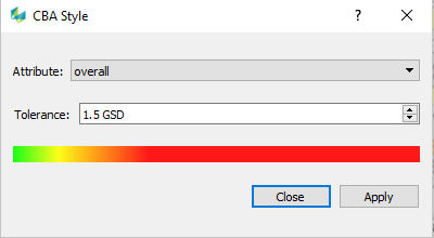
The reference value for color codes can be set using the Layer tab. It allows to provide a GSD factor, which serves as reference threshold. Threshold can be set per horizontal or vertical component.

To set the threshold to use, right-click on the CBA layer and select “Edit CBA Style”.

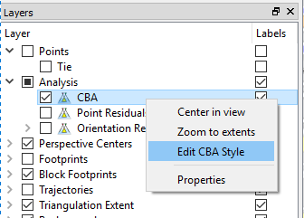
It is then possible to change both attribute to use as well as define the tolerance.

Point residuals

Allow to visualize the residuals of control points in the map view:

• horizontal object residuals are shown as a vector

• vertical object residuals are shown as a circle

Orientation residuals

Allow to visualize the residuals of projection center:

• horizontal object residuals are shown as a vector

• vertical object residuals are shown as a circle

• angular object residuals can be visualized

Filters for Analysis

A very helpful tool during analysis of the Aerotriangulation results is the filter tool. Filter selection can be opened via View > Filters.

The tool affects the display in the map view and point list and therefore makes interpretation and selection tasks easier. Often used filters can be saved and are available as listed items.

Samples for the use of filters are listed below:

Display per Ray

Display per Residual

Display tie points, where image measurements residuals are between 0.5 and 1 pixel.